Arrays vs. Linked Lists: Proposing a Hybrid Approach
Introduction
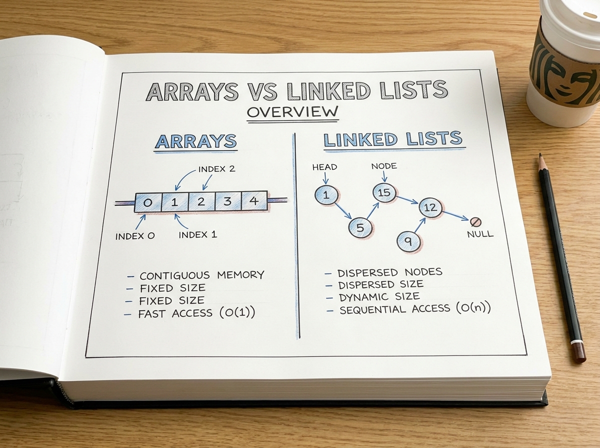
Data structures are one of the most fundamental building blocks in computer science. Among them, arrays and linked lists are often introduced as two completely different approaches for storing and managing data. Arrays provide fast random access and excellent cache locality, while linked lists offer flexible memory usage and efficient insertions or deletions.
However, both structures come with significant tradeoffs.
Arrays rely on contiguous memory allocation, which makes resizing expensive and insertions inefficient for large datasets. Linked lists solve some of these issues through dynamic node allocation, but they suffer from poor cache performance, additional pointer overhead, and slower traversal speed.
In real-world systems, choosing between arrays and linked lists is rarely straightforward. High-performance applications often require both efficient memory access and dynamic modification capabilities at the same time. This naturally raises an important question:
Is it possible to combine the strengths of arrays and linked lists while minimizing their weaknesses?
In this article, we will first examine how arrays and linked lists work internally, analyze their advantages and limitations, and then explore a proposed hybrid approach that attempts to balance memory efficiency, traversal performance, and structural flexibility.
Rather than treating arrays and linked lists as competing structures, this discussion aims to investigate whether they can instead complement each other in a more optimized design.
Internal Structure
Arrays
An array is a linear data structure in which elements are stored in contiguous memory locations. This means that each element is placed directly next to the previous one in memory. Because of this predictable memory layout, arrays provide extremely fast access to elements using their index.
For example, consider the following integer array:
int arr[5] = {10, 20, 30, 40, 50};
If the base address of the array is known, the memory address of any element can be calculated mathematically using:
Address(arr[i]) = Base Address + (i × Size of Element)
This direct address computation is what allows arrays to achieve constant-time random access:
Access Complexity: O(1)
Unlike some other data structures, arrays do not require traversal from one element to another in order to access data. The processor can directly jump to the required memory location.
Memory Layout
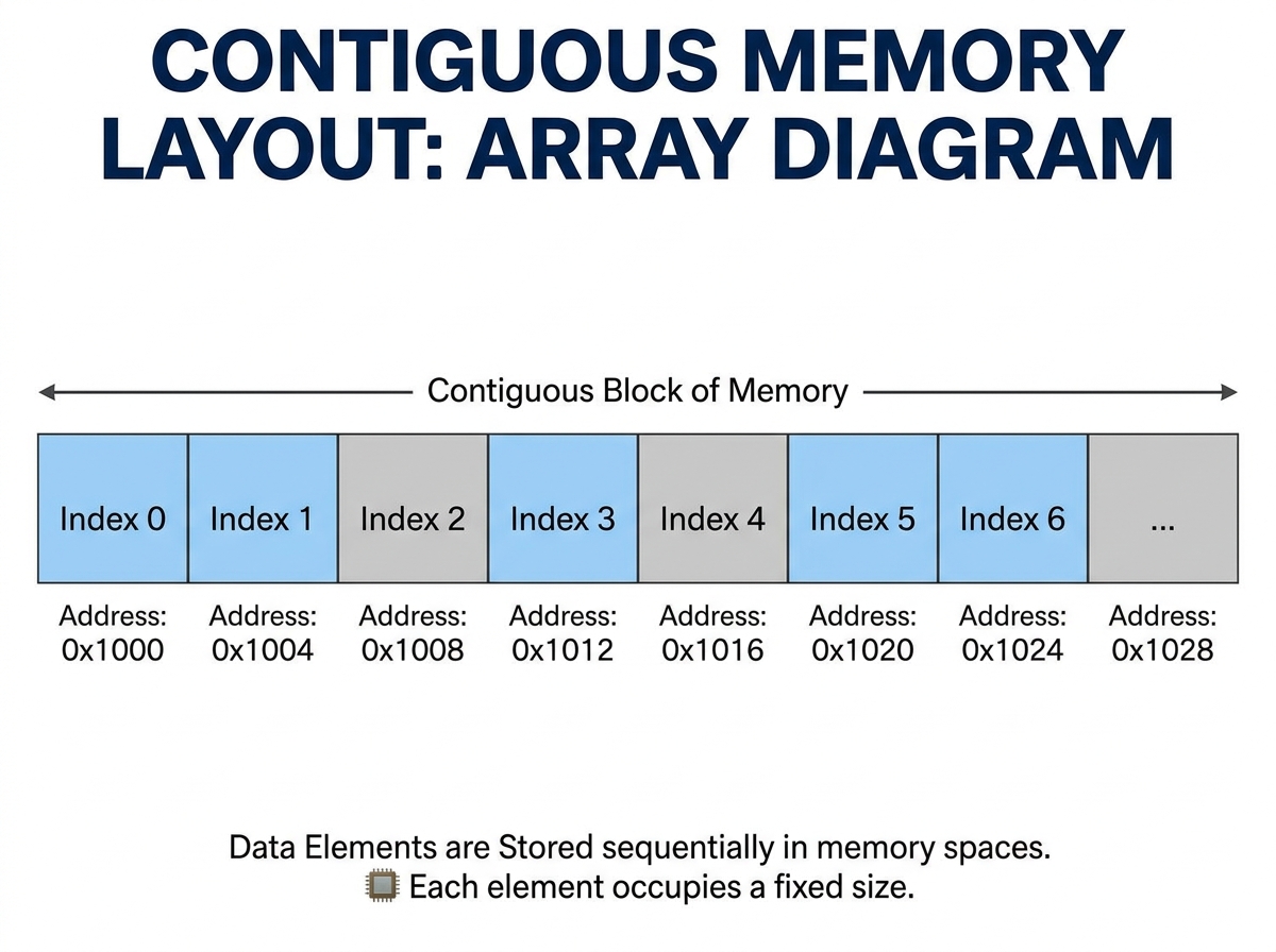
A simplified representation of an array in memory looks like this:
Index:      0     1     2     3     4
Value:     10    20    30    40    50

Memory:
+----+----+----+----+----+
| 10 | 20 | 30 | 40 | 50 |
+----+----+----+----+----+
Since the elements are tightly packed together, arrays are highly cache-friendly. Modern CPUs load nearby memory locations into cache lines, meaning sequential array traversal benefits significantly from spatial locality.
This is one of the primary reasons arrays often outperform linked lists in practical applications, even when theoretical time complexities appear similar.
Advantages of Arrays
Arrays provide several important advantages:
- Fast random access through indexing
- Excellent cache locality
- Minimal memory overhead
- Efficient sequential traversal
- Simple memory representation
Because of these characteristics, arrays are widely used in:
- matrices,
- buffers,
- lookup tables,
- heaps,
- dynamic programming tables,
- and many low-level system components.
Limitations of Arrays
Despite their strengths, arrays also introduce important constraints.
Fixed Size Limitation
Traditional arrays require a predefined size during allocation:
int arr[100];
If the allocated size becomes insufficient, resizing usually requires:
- allocating a larger memory block,
- copying existing elements,
- and releasing the old memory.
This resizing operation can become expensive for large datasets.
Expensive Insertions and Deletions
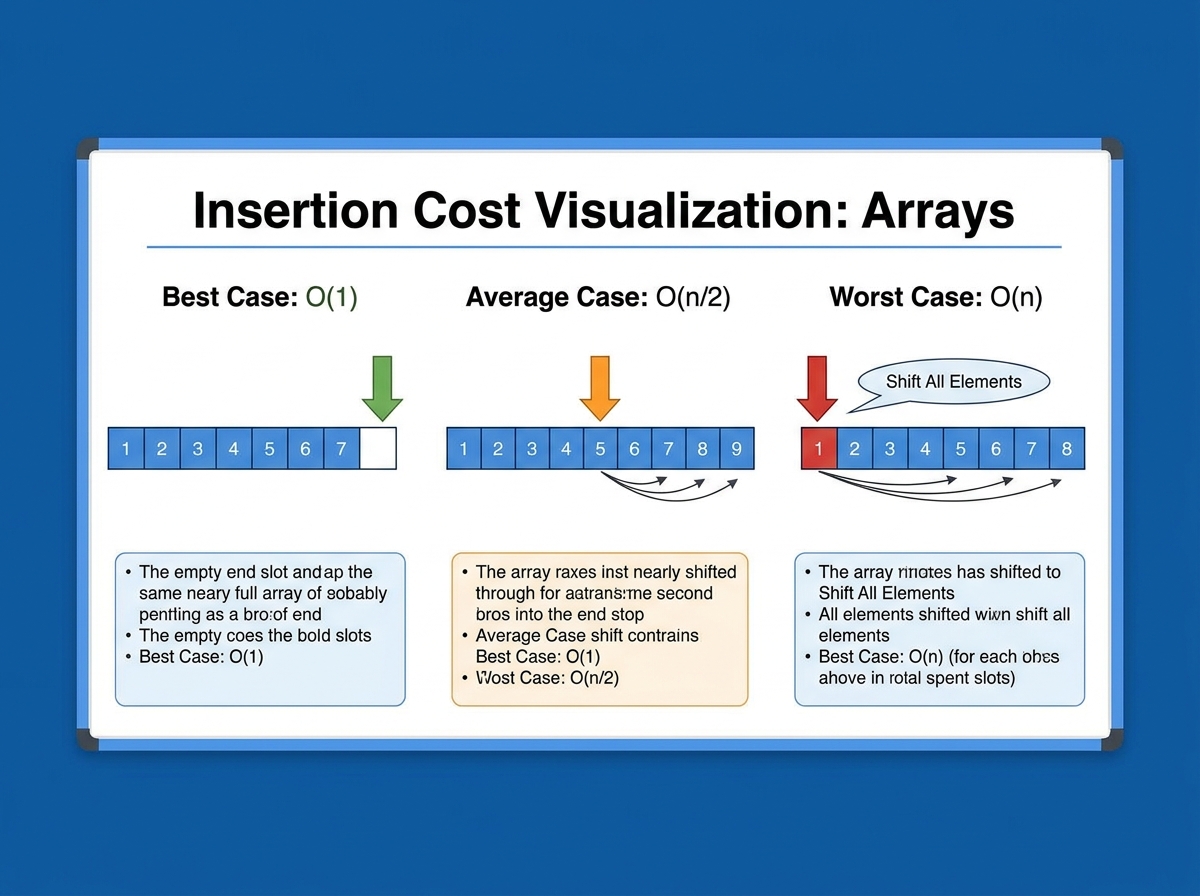
Insertion or deletion in the middle of an array requires shifting elements:
Before Insertion:
[10, 20, 40, 50]

Insert 30 at index 2

After Insertion:
[10, 20, 30, 40, 50]
In the worst case, this shifting operation takes:
Insertion Complexity: O(n)
Deletion Complexity: O(n)
Contiguous Memory Requirement
Since arrays require contiguous memory allocation, extremely large arrays may face allocation difficulties in fragmented memory environments.
This becomes particularly relevant in:
- embedded systems,
- memory-constrained environments,
- and low-level system programming.
As datasets grow dynamically, the rigidity of arrays begins to expose their limitations, motivating the need for more flexible structures such as linked lists.
Linked Lists
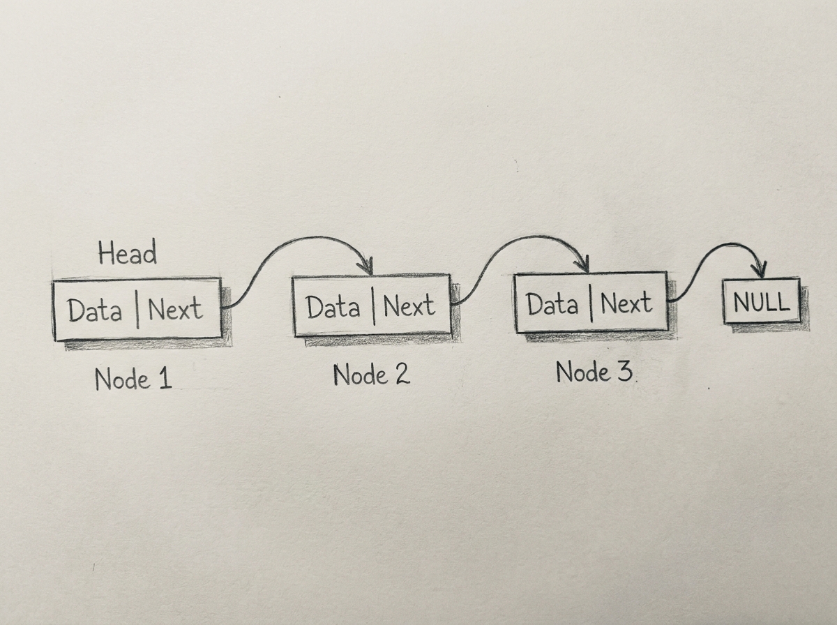
Unlike arrays, linked lists do not store elements in contiguous memory locations. Instead, a linked list consists of multiple individual nodes distributed dynamically throughout memory. Each node stores two primary components:
- The actual data
- A pointer (or reference) to the next node
This pointer-based structure allows linked lists to grow and shrink dynamically without requiring contiguous memory allocation.
A simplified singly linked list node can be represented as:
struct Node
{
    int data;
    Node* next;
};
Each node maintains a connection to the next node in the sequence, forming a chain-like structure:
+----+------+    +----+------+    +----+------+
| 10 |  *---|--->| 20 |  *---|--->| 30 | NULL |
+----+------+    +----+------+    +----+------+
Unlike arrays, linked lists do not support direct indexing because nodes may exist at completely unrelated memory locations.
To access a particular element, traversal must begin from the head node and proceed sequentially until the desired node is reached.
Access Complexity: O(n)
Memory Layout
Unlike arrays, linked list nodes are often scattered throughout memory rather than being stored sequentially.
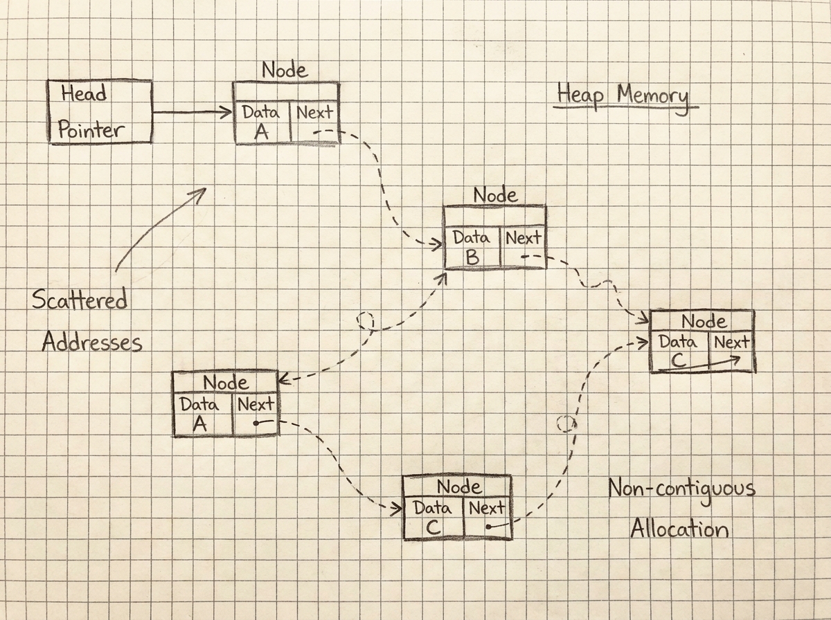
A conceptual representation may look like this:
Node 1 -> Address 1000
Node 2 -> Address 8040
Node 3 -> Address 2230
Node 4 -> Address 9100
This scattered allocation introduces one of the biggest practical disadvantages of linked lists: poor cache locality.
Modern CPUs are heavily optimized for sequential memory access. Since linked list nodes may be distributed unpredictably across memory, traversing a linked list often results in frequent cache misses and reduced processor efficiency.
This is one reason why linked lists can perform significantly slower than arrays in real-world applications despite offering efficient insertion and deletion operations.
Advantages of Linked Lists
Linked lists provide several important advantages over arrays.
Dynamic Size
Linked lists can grow and shrink dynamically during runtime without requiring large contiguous memory blocks.
New nodes can simply be allocated whenever additional storage is required.
Efficient Insertions and Deletions
One of the strongest advantages of linked lists is the ability to perform insertions and deletions efficiently without shifting large amounts of data.
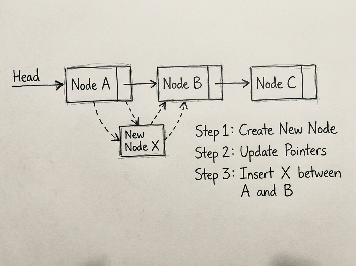
For example:
Before:
10 -> 20 -> 40

After inserting 30:
10 -> 20 -> 30 -> 40
In many cases, only pointer adjustments are required.
Insertion Complexity: O(1)
Deletion Complexity: O(1)
This efficiency becomes especially valuable in:
- dynamic memory systems,
- scheduling systems,
- graph structures,
- memory allocators,
- and operating system internals.
Flexible Memory Usage
Because linked lists allocate memory node-by-node, they can operate effectively even in fragmented memory environments where large contiguous blocks are unavailable.
Limitations of Linked Lists
Despite their flexibility, linked lists also introduce several important drawbacks.
Poor Random Access
Unlike arrays, linked lists cannot directly jump to a specific element.
To access the nth element, traversal must proceed sequentially from the beginning:
Traversal:
Head -> Node1 -> Node2 -> Node3 -> ...
This makes random access significantly slower.
Random Access Complexity: O(n)
Additional Memory Overhead
Each node requires extra storage for pointers:
struct Node
{
    int data;
    Node* next;
};
For very large datasets, this pointer overhead can become substantial.
Poor Cache Performance
Since nodes are scattered throughout memory, linked lists suffer from:
- cache misses,
- pointer chasing,
- and reduced spatial locality.
In modern processor architectures, this often causes linked lists to perform worse than arrays for traversal-heavy workloads.
Increased Structural Complexity
Compared to arrays, linked lists require:
- dynamic memory management,
- pointer manipulation,
- and careful handling of edge cases.
Improper pointer handling may lead to:
- memory leaks,
- dangling pointers,
- segmentation faults,
- and structural corruption.
As a result, linked lists trade memory locality and simplicity for flexibility and dynamic modification capabilities.
Motivation for a Hybrid Approach
Arrays and linked lists are often presented as fundamentally different data structures, each optimized for a different set of problems. Arrays prioritize fast access and memory locality, while linked lists prioritize structural flexibility and efficient modifications.
However, when examined closely, neither structure is universally optimal.
Arrays excel at:
- sequential traversal,
- random access,
- and cache-efficient computation.
But they struggle with:
- dynamic resizing,
- middle insertions,
- deletions,
- and contiguous memory requirements.
On the other hand, linked lists solve many of these modification-related issues through dynamic node allocation. Insertions and deletions can often be performed without shifting large amounts of data. However, this flexibility comes at the cost of:
- poor cache locality,
- increased pointer overhead,
- fragmented memory access,
- and slower traversal performance.
This creates an important tradeoff in practical system design.
Many real-world applications require both:
- efficient traversal performance,
- and dynamic structural modifications.
Unfortunately, arrays and linked lists individually optimize only one side of this problem.
For example:
- Arrays are highly efficient for read-heavy workloads but inefficient for frequent modifications.
- Linked lists handle structural changes efficiently but suffer in traversal-intensive operations.
This limitation becomes increasingly visible in:
- database engines,
- memory allocators,
- file systems,
- graph processing systems,
- scheduling systems,
- and high-performance computing applications.
In modern computer architectures, memory access patterns have become just as important as theoretical time complexity. A data structure with better cache behavior can often outperform another structure even if both share similar asymptotic complexity.
For instance, although linked lists provide efficient insertions in theory, their scattered memory layout can significantly degrade real-world performance due to:
- cache misses,
- pointer chasing,
- and reduced spatial locality.
This naturally leads to an important design question:
Can a data structure preserve the cache efficiency of arrays while also maintaining some of the flexibility offered by linked lists?
A hybrid approach attempts to explore this possibility.
Instead of viewing arrays and linked lists as competing structures, a hybrid model attempts to combine their strengths into a more balanced design. The objective is not necessarily to completely eliminate their weaknesses, but rather to reduce the severity of their tradeoffs.
Such a structure could potentially:
- improve cache locality compared to linked lists,
- reduce insertion costs compared to arrays,
- minimize memory fragmentation,
- and maintain better scalability for dynamically changing datasets.
The following sections explore one possible hybrid design that attempts to achieve this balance.
Dynamic Arrays
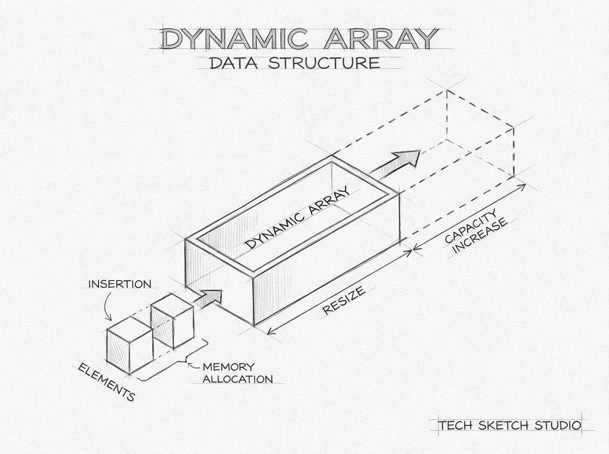
A dynamic array is an advanced form of array that can automatically resize itself during runtime.
Unlike static arrays, dynamic arrays are not restricted to a fixed capacity.
Popular examples include:
std::vectorin C++ArrayListin Javalistin Python (internally dynamic array based)
How Dynamic Arrays Solve the Problem of Static Arrays
Suppose we create a static array of size 4.
int arr[4];
Once all four positions are occupied, no additional element can be inserted.
Dynamic arrays solve this by automatically allocating a larger memory block whenever the current storage becomes full.
Instead of failing immediately, the container performs:
- Allocate a new larger memory block
- Copy old elements into the new block
- Free old memory
- Continue insertion normally
This process is called:
Resizing
Why Dynamic Arrays Usually Double Their Size
Most dynamic arrays increase their capacity by a factor of 2.
Example:
| Current Capacity | New Capacity |
|---|---|
| 2 | 4 |
| 4 | 8 |
| 8 | 16 |
| 16 | 32 |
This strategy is used because repeatedly increasing by only 1 would cause excessive reallocations.
Example of Resizing
Suppose a dynamic array currently has:
Capacity = 4
Size = 4
Current layout:
[10][20][30][40]
Now we insert another element:
push_back(50)
Since capacity is full:
- A new array of size
8is allocated - Existing elements are copied
- Old array memory is released
- New element is inserted
Result:
[10][20][30][40][50]
New state:
Capacity = 8
Size = 5
Why Doubling is Efficient
Doubling significantly reduces the number of expensive resizing operations.
If capacity increased by only 1 every time:
1 → 2 → 3 → 4 → 5 → 6 ...
then every insertion near full capacity would require:
- new allocation
- full copying
- memory deallocation
This becomes extremely slow.
With doubling:
1 → 2 → 4 → 8 → 16 → 32 ...
the number of reallocations becomes much smaller.
This gives dynamic arrays an important property:
Amortized O(1) insertion at the end.
Even though occasional resizing is expensive, most insertions remain extremely fast.
Advantages of Dynamic Arrays Over Static Arrays
1. Automatic Resizing
Dynamic arrays grow automatically during runtime.
No need to predict exact data size beforehand.
2. Better Memory Utilization
Memory grows according to demand instead of allocating excessively large fixed arrays initially.
3. Fast Random Access
Just like static arrays, dynamic arrays support:
O(1)
index-based access because memory remains contiguous.
Example:
arr[i]
remains extremely efficient.
4. Cache Friendly
Since elements are stored contiguously:
- CPU cache utilization improves
- Traversal becomes faster
- Sequential processing becomes highly optimized
This is one reason arrays outperform linked lists in many practical systems.
5. Simplified Development
Developers do not need to manually manage resizing logic repeatedly.
Modern containers handle allocation internally.
Limitations of Dynamic Arrays
Although dynamic arrays solve several issues of static arrays, they still inherit some array-related limitations.
1. Expensive Resizing Operation
Whenever resizing occurs:
- New memory allocation happens
- All elements must be copied
- Old memory is released
For large datasets, this operation becomes costly.
Time complexity during resizing:
O(n)
2. Slow Insertions in Middle
Inserting elements in the middle requires shifting elements.
Example:
[10][20][30][40]
Insert 25 at index 2:
[10][20][25][30][40]
Elements after insertion point must move.
Complexity:
O(n)
3. Slow Deletions in Middle
Deleting elements also requires shifting remaining elements.
Example:
[10][20][30][40]
Delete 20:
[10][30][40]
Again, shifting occurs.
Complexity:
O(n)
4. Requires Contiguous Memory
Dynamic arrays still require contiguous memory allocation.
For extremely large arrays, finding large contiguous blocks may become difficult in fragmented memory systems.
Recommended Use Cases for Dynamic Arrays
Dynamic arrays are excellent when:
1. Frequent Random Access is Needed
Example:
- Index-based retrieval
- Matrix operations
- Lookup tables
- Image processing
Because access remains:
O(1)
2. Most Insertions Occur at the End
Example:
- Stack implementations
- Logging systems
- Appending data streams
- Dynamic buffers
Appending is highly optimized.
3. Cache Performance Matters
Dynamic arrays are preferred in:
- Game engines
- Numerical computing
- Competitive programming
- Scientific simulations
because contiguous memory improves hardware-level performance.
When Dynamic Arrays Are NOT Recommended
Dynamic arrays are not ideal when:
1. Frequent Insertions/Deletions Occur in Middle
Example:
- Text editors
- Real-time queue manipulation
- Frequent reordering systems
Because shifting becomes expensive.
Linked lists often perform better in such scenarios.
2. Stable Memory Addresses Are Required
Resizing changes the underlying memory location.
Pointers/references to old elements may become invalid after reallocation.
This can create serious issues in low-level systems programming.
3. Extremely Large Continuous Allocations Are Problematic
Systems with fragmented memory may struggle to allocate very large contiguous blocks.
Linked structures become more flexible in such environments.
Dynamic Arrays: A Hybrid Philosophy
Dynamic arrays represent a hybrid balance between:
| Array Strengths | Added Flexibility |
|---|---|
| Fast access | Runtime resizing |
| Cache efficiency | Automatic growth |
| Simple indexing | Better usability |
They preserve most advantages of arrays while reducing one of the biggest weaknesses of static allocation.
However, they still cannot efficiently solve problems involving heavy insertion and deletion operations in arbitrary positions.
This limitation eventually motivates the need for linked data structures such as linked lists.
Skip Lists
As software systems evolved, developers discovered that neither arrays nor linked lists were universally optimal.
Arrays provided:
- Fast random access
- Excellent cache locality
- Efficient traversal
but suffered from:
- Expensive insertions/deletions in middle
- Costly resizing operations
- Requirement of contiguous memory
Linked lists solved several of these problems by allowing:
- Dynamic memory allocation
- Efficient insertions and deletions
- Flexible memory usage
However, linked lists introduced an entirely new issue:
Slow searching.
Searching inside a linked list requires sequential traversal.
Time complexity:
O(n)
This became inefficient for large datasets.
To overcome this limitation while preserving linked-list flexibility, a powerful probabilistic data structure was introduced:
Skip List
What is a Skip List?
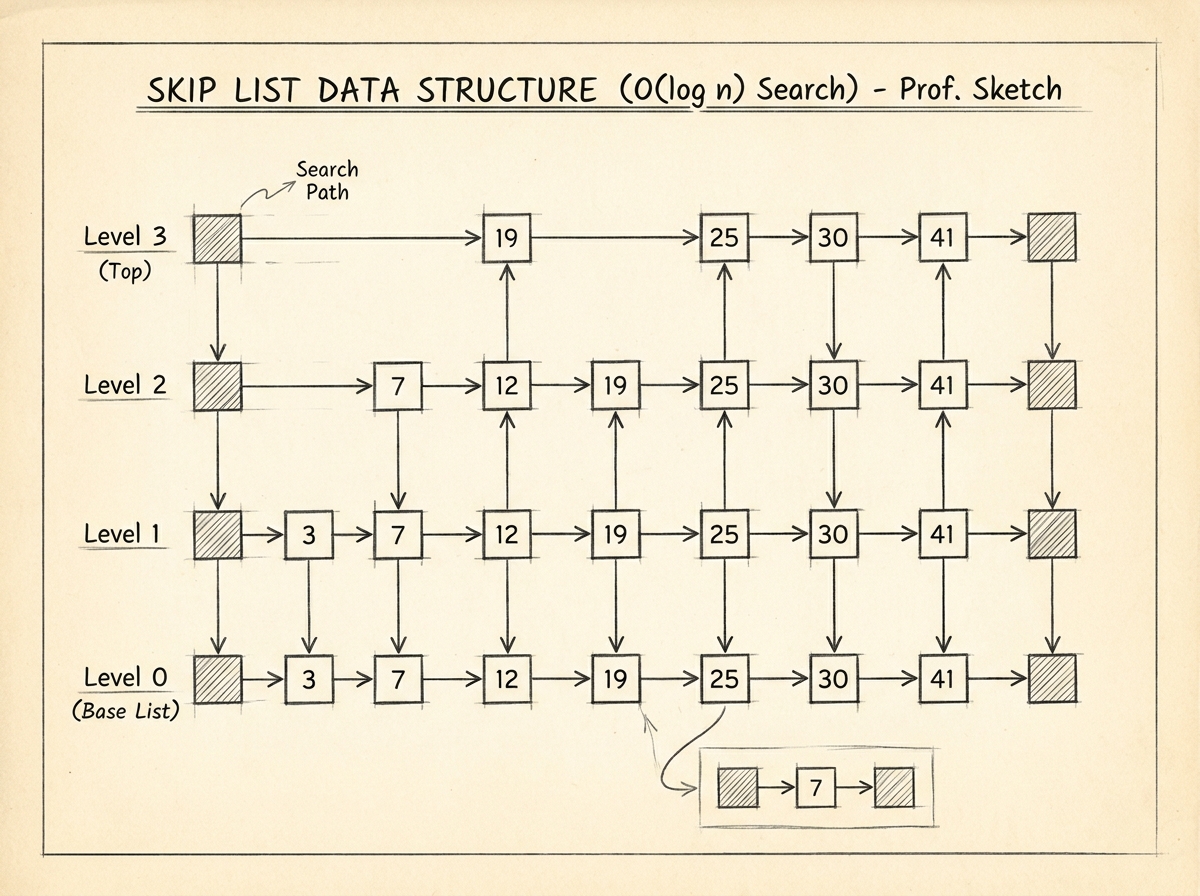
A skip list is an advanced layered linked-list structure designed to speed up searching operations.
Instead of traversing nodes one-by-one like a normal linked list, skip lists create multiple shortcut layers that allow the algorithm to “skip” over large portions of the data.
This dramatically improves searching efficiency.
Average complexities become:
| Operation | Complexity |
|---|---|
| Search | O(log n) |
| Insertion | O(log n) |
| Deletion | O(log n) |
Core Idea Behind Skip Lists
A normal linked list looks like this:
1 → 2 → 3 → 4 → 5 → 6 → 7 → 8
To search for 8, traversal must visit nearly every node.
Skip lists improve this by introducing higher-level shortcut links.
Example conceptual structure:
Level 2: 1 ----------- 5 ----------- 8
Level 1: 1 ----- 3 ----- 5 ----- 7 ----- 8
Level 0: 1 - 2 - 3 - 4 - 5 - 6 - 7 - 8
Higher levels allow traversal to jump faster across the structure.
Instead of scanning sequentially:
1 → 2 → 3 → 4 → 5 → 6 → 7 → 8
search may become:
1 → 5 → 7 → 8
This significantly reduces traversal cost.
How Skip Lists Solve the Problems of Linked Lists
Traditional linked lists suffer from poor searching performance.
Example:
Search = O(n)
because traversal is sequential.
Skip lists solve this by adding:
- Multiple hierarchical levels
- Shortcut pointers
- Faster traversal paths
This transforms searching into approximately:
O(log n)
which becomes dramatically faster for large datasets.
How Skip Lists Compare Against Arrays
Arrays provide fast searching only when:
- Binary search is applicable
- Data is sorted
- Insertions/deletions are infrequent
However, arrays still suffer from:
- Expensive shifting operations
- Resizing overhead
- Contiguous memory dependency
Skip lists avoid these problems because:
- Nodes are dynamically allocated
- Insertions do not require shifting
- Deletions do not require moving elements
- Memory can grow flexibly
This makes skip lists a hybrid balance between:
| Array Strength | Linked List Strength |
|---|---|
| Fast searching | Dynamic flexibility |
| Logarithmic traversal | Efficient modifications |
How Searching Works in a Skip List
Searching starts from the highest level.
The algorithm:
- Move forward while values remain smaller than target
- Drop one level when forward movement is no longer possible
- Repeat until bottom level is reached
Example search for 7:
Top Level:
1 -------- 5 -------- 8
             ↓

Middle Level:
5 ----- 7 ----- 8
        ↓

Bottom Level:
7
Instead of visiting every node, the structure intelligently skips sections.
Randomized Level Generation
One unique feature of skip lists is probabilistic balancing.
When a new node is inserted:
- Random coin flips determine how many levels the node receives
- Some nodes appear only in lower levels
- Few nodes appear in higher levels
This creates a naturally balanced structure without requiring complex tree rotations.
Advantages of Skip Lists
1. Fast Searching
Skip lists provide near-balanced-tree performance.
Average search complexity:
O(log n)
which is significantly faster than linked lists.
2. Efficient Insertions and Deletions
Unlike arrays:
- No element shifting is required
- No resizing is necessary
- Operations remain efficient
Average complexities:
Insertion = O(log n)
Deletion = O(log n)
3. Simpler Than Balanced Trees
Balanced trees such as:
- AVL Trees
- Red-Black Trees
require:
- Rotations
- Rebalancing logic
- Complex implementation
Skip lists achieve comparable average performance with much simpler logic.
This makes implementation easier.
4. Dynamic Memory Allocation
Like linked lists, skip lists allocate memory dynamically.
No large contiguous memory block is required.
This improves flexibility in fragmented memory environments.
5. Excellent for Ordered Data
Skip lists maintain sorted order naturally.
This makes them useful for:
- Databases
- Indexing systems
- Ordered caches
- In-memory storage engines
6. Concurrent-Friendly Structure
Skip lists are often easier to optimize for concurrent systems compared to balanced trees.
Many modern databases and distributed systems use skip lists because:
- Node-level modifications are localized
- Parallel operations become easier
- Lock contention can be reduced
Limitations of Skip Lists
Despite their strengths, skip lists are not perfect.
1. Higher Memory Usage
Each node may contain multiple forward pointers.
Example:
Node:
[value | level1 | level2 | level3]
This increases memory consumption compared to ordinary linked lists.
2. Cache Locality is Poorer Than Arrays
Arrays store elements contiguously.
Skip lists use dynamically scattered nodes.
This leads to:
- More cache misses
- Reduced traversal locality
- Higher pointer-chasing overhead
In many real systems, arrays can still outperform skip lists despite worse theoretical insertion complexity.
3. Worst-Case Complexity Still Exists
Although average performance is:
O(log n)
worst-case performance may degrade toward:
O(n)
if level distribution becomes highly unbalanced.
However, good probabilistic balancing makes this rare.
4. Randomization May Be Undesirable
Some systems require deterministic guarantees.
Since skip lists depend on probabilistic balancing:
- Performance may vary slightly
- Structure is not strictly deterministic
In such cases, balanced trees may be preferred.
When Should You Prefer Skip Lists?
Skip lists are highly suitable when:
1. Frequent Searching + Frequent Insertions/Deletions
Example:
- Dynamic ordered datasets
- Real-time indexing
- Event scheduling systems
because skip lists efficiently support all operations together.
2. Simpler Alternative to Balanced Trees is Needed
If you want:
- Logarithmic performance
- Easier implementation
- Reduced balancing complexity
skip lists become an excellent option.
3. Concurrent Systems
Skip lists are commonly used in:
- Distributed databases
- Concurrent caches
- Multi-threaded storage systems
because their structure adapts well to parallel operations.
4. Ordered Data Structures
Skip lists naturally maintain sorted order while supporting efficient updates.
Useful in:
- Ranking systems
- Leaderboards
- Search indexing
- Ordered maps
When Skip Lists Are NOT Recommended
Skip lists are not ideal when:
1. Maximum Cache Efficiency is Required
Arrays still dominate in:
- Numerical computation
- Scientific simulation
- GPU-style workloads
- High-performance contiguous traversal
because arrays exploit hardware caching much better.
2. Memory Usage Must Be Minimal
Extra pointers increase memory overhead.
For highly memory-constrained systems, skip lists may become expensive.
3. Deterministic Worst-Case Guarantees Are Required
Systems requiring strict guarantees may prefer:
- AVL Trees
- Red-Black Trees
- B-Trees
because their balancing is deterministic.
Skip Lists: A True Hybrid Structure
Skip lists combine several important characteristics together:
| Capability | Source |
|---|---|
| Dynamic allocation | Linked Lists |
| Efficient insertion/deletion | Linked Lists |
| Fast logarithmic search | Balanced Trees |
| Simpler implementation | Probabilistic design |
They act as a bridge between:
- linked lists
- balanced trees
- ordered indexing systems
Skip lists demonstrate an important idea in data structure design:
Sometimes probabilistic simplicity can outperform deterministic complexity in practical systems.
They are one of the most elegant examples of hybrid data-structure engineering.
Unrolled Linked Lists
As developers continued exploring the trade-offs between arrays and linked lists, another important observation emerged:
Traditional linked lists solve the insertion and deletion problems of arrays, but they introduce serious inefficiencies such as:
- Poor cache locality
- High memory overhead due to pointers
- Slow traversal performance
- Increased memory fragmentation
Arrays, on the other hand, provide:
- Excellent cache performance
- Compact memory layout
- Fast traversal
but still suffer from:
- Expensive insertions/deletions
- Shifting operations
- Resizing costs
This motivated the development of a hybrid structure designed to combine:
- the flexibility of linked lists
- the locality benefits of arrays
The result was:
Unrolled Linked List
What is an Unrolled Linked List?
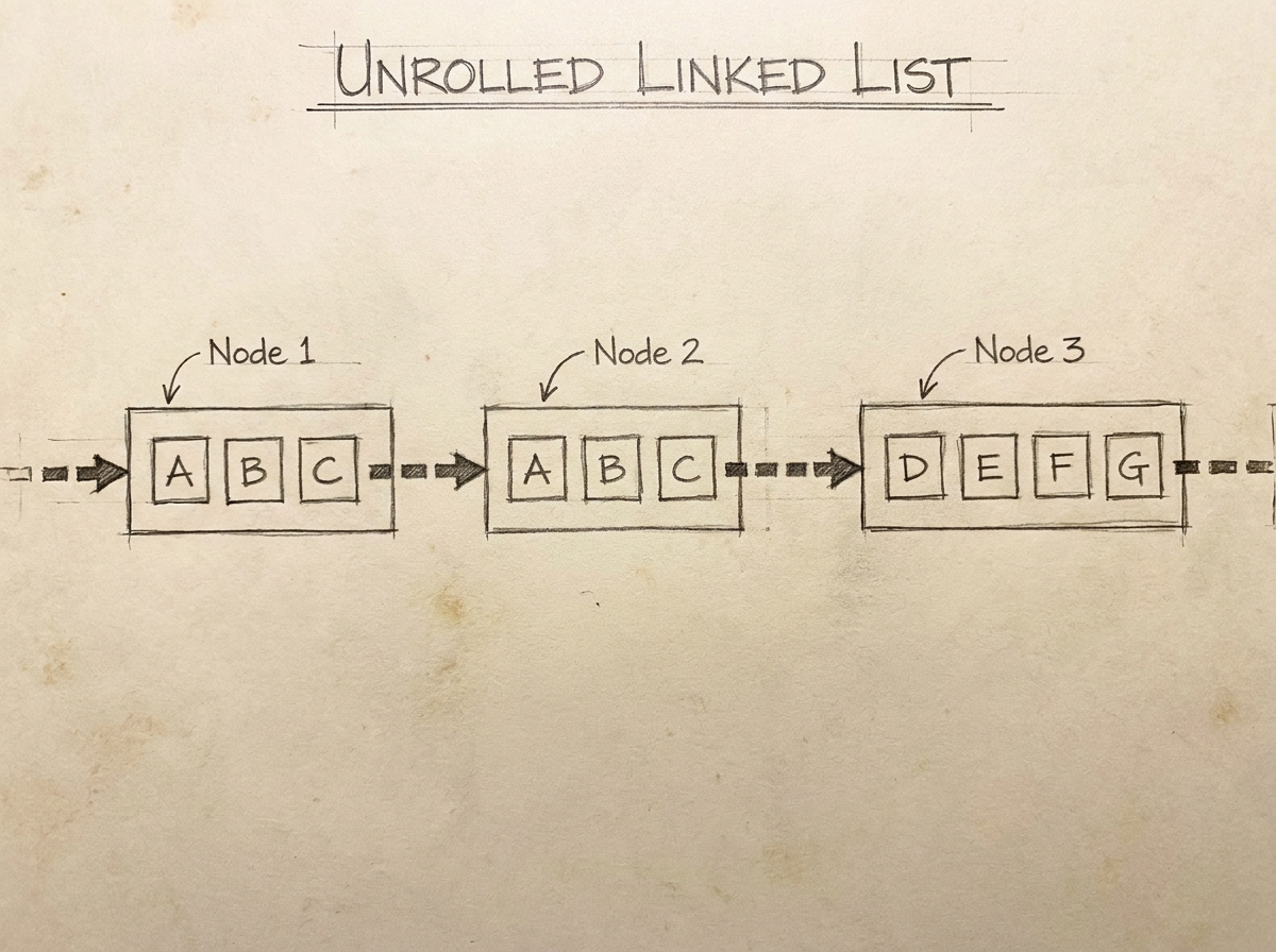
An unrolled linked list is an advanced variation of a linked list where:
Each node stores multiple elements instead of storing only one element.
Instead of this traditional linked list structure:
[A] → [B] → [C] → [D]
an unrolled linked list stores blocks of elements:
[A B C] → [D E F] → [G H I]
Each node internally behaves like a small array.
This reduces:
- pointer overhead
- memory fragmentation
- traversal cost
while still preserving linked-list flexibility.
Core Idea Behind Unrolled Linked Lists
A standard linked list allocates one node per element:
[value | next]
This creates several inefficiencies:
- Large number of pointer objects
- Scattered memory allocation
- Poor CPU cache utilization
Unrolled linked lists solve this by grouping multiple elements together inside a node.
Example node structure:
Node:
[10 20 30 40] → next
Now fewer nodes are required for the same amount of data.
This improves:
- cache locality
- traversal efficiency
- memory utilization
How Unrolled Linked Lists Solve Problems of Traditional Linked Lists
Traditional linked lists suffer from:
1. Excessive Pointer Overhead
Normal linked lists require one pointer per element.
Example:
[value | next]
For very large datasets, pointer memory becomes substantial.
Unrolled linked lists reduce the total number of nodes.
Example:
Instead of:
[A] → [B] → [C] → [D]
we get:
[A B C D]
This drastically reduces pointer overhead.
2. Poor Cache Locality
Linked-list nodes are scattered throughout memory.
This causes:
- frequent cache misses
- slower traversal
- poor hardware utilization
Unrolled linked lists improve locality because multiple nearby elements are stored contiguously inside the same node.
This allows CPUs to process data more efficiently.
3. Slow Sequential Traversal
Traditional linked lists require pointer traversal for every element.
Unrolled linked lists reduce the number of pointer jumps significantly.
Traversal becomes much faster because:
- several elements are processed per node visit
- fewer memory dereferences occur
How Unrolled Linked Lists Compare Against Arrays
Arrays provide:
- compact contiguous storage
- excellent cache performance
- fast indexing
but suffer from:
- expensive insertions/deletions
- shifting operations
- resizing costs
Unrolled linked lists partially solve these issues by:
- allowing dynamic node allocation
- reducing large-scale shifting
- supporting efficient insertions/deletions
while still maintaining better locality than ordinary linked lists.
This creates a hybrid balance between:
| Array Strength | Linked List Strength |
|---|---|
| Cache efficiency | Dynamic allocation |
| Compact storage | Flexible insertions |
| Better traversal speed | Easier modifications |
Structure of an Unrolled Linked List
Each node contains:
- an internal array
- current element count
- pointer to next node
Example:
Node 1:
[10 20 30 40]

Node 2:
[50 60 70 80]
Conceptually:
[10 20 30 40] → [50 60 70 80]
Each node behaves like a mini-array.
How Insertions Work
Suppose node capacity is:
4 elements
Current structure:
[10 20 30 40] → [50 60]
Now insert:
25
The node may:
- shift elements internally
- split into another node if full
Example after split:
[10 20] → [25 30 40] → [50 60]
This resembles concepts used in:
- B-Trees
- Block-based storage systems
Advantages of Unrolled Linked Lists
1. Better Cache Performance
Since multiple elements are stored contiguously:
- cache locality improves
- traversal becomes faster
- CPU prefetching becomes more effective
This is one of the biggest improvements over ordinary linked lists.
2. Reduced Pointer Overhead
Fewer nodes mean:
- fewer pointers
- lower metadata overhead
- improved memory efficiency
Compared to traditional linked lists, this becomes highly beneficial for massive datasets.
3. Faster Traversal
Instead of dereferencing a pointer for every single element:
A → B → C → D
the algorithm processes multiple elements together:
[A B C D]
This significantly reduces traversal cost.
4. Dynamic Flexibility
Like linked lists:
- nodes can be added dynamically
- contiguous global memory is not required
- resizing large arrays is avoided
This preserves flexibility.
5. Efficient Insertions and Deletions
Compared to arrays:
- large-scale shifting is avoided
- modifications remain localized
- operations become more flexible
especially for mid-sized dynamic datasets.
6. Useful in Memory-Constrained Systems
Because pointer overhead is reduced, unrolled linked lists may become more memory-efficient than ordinary linked lists.
This becomes useful in:
- embedded systems
- storage engines
- memory-sensitive applications
Limitations of Unrolled Linked Lists
Despite their strengths, unrolled linked lists also introduce several trade-offs.
1. More Complex Implementation
Compared to ordinary linked lists:
- node splitting logic is needed
- balancing node occupancy becomes necessary
- insertions become more complicated
Implementation complexity increases substantially.
2. Random Access is Still Slow
Unlike arrays:
arr[i]
cannot be accessed directly in constant time.
Traversal is still required.
Complexity remains approximately:
O(n)
although traversal constants improve.
3. Internal Shifting Still Exists
Within a node, insertions/deletions may still require shifting elements.
Example:
[10 20 30 40]
Insert 25:
[10 20 25 30 40]
Internal movement still occurs.
4. Node Splitting Overhead
When nodes become full:
- splitting operations occur
- elements may redistribute
- additional allocations become necessary
This introduces extra complexity.
5. Cache Performance Still Inferior to Arrays
Although significantly better than linked lists, unrolled linked lists still cannot fully match arrays because:
- nodes remain scattered globally
- pointer traversal still exists
- perfect contiguity is absent
Arrays remain superior for maximum hardware efficiency.
When Should You Prefer Unrolled Linked Lists?
Unrolled linked lists are highly useful when:
1. Frequent Traversal + Frequent Modifications Are Needed
They perform well when applications require both:
- dynamic insertions/deletions
- efficient sequential traversal
2. Linked List Pointer Overhead Becomes Problematic
For extremely large linked structures, reducing pointer count can significantly improve performance and memory usage.
3. Cache Efficiency Matters but Arrays Are Too Rigid
Unrolled linked lists provide a compromise between:
- array locality
- linked-list flexibility
This becomes useful in practical systems.
4. Block-Oriented Processing is Beneficial
Applications involving grouped processing often benefit from node-level batching.
Examples:
- text editors
- memory allocators
- storage engines
- buffering systems
5. Dynamic Datasets with Moderate Insertions
When insertions occur frequently but complete array shifting becomes too expensive, unrolled linked lists provide a balanced solution.
When Unrolled Linked Lists Are NOT Recommended
Unrolled linked lists are not ideal when:
1. True Constant-Time Random Access is Required
Arrays remain far superior for direct indexing operations.
Example:
arr[i]
cannot be efficiently replicated.
2. Maximum Simplicity is Desired
Traditional arrays and linked lists are significantly easier to implement and debug.
Unrolled linked lists introduce:
- node balancing
- occupancy management
- split handling
which increase complexity.
3. Data Size is Small
For small datasets, the additional complexity often provides negligible practical benefit.
Simple structures become preferable.
4. Strict Real-Time Predictability is Required
Node splitting and redistribution may create inconsistent operation costs.
Systems requiring tightly bounded execution times may prefer more deterministic structures.
Unrolled Linked Lists: A Hybrid Storage Strategy
Unrolled linked lists combine important characteristics from both arrays and linked lists:
| Capability | Source |
|---|---|
| Dynamic memory allocation | Linked Lists |
| Reduced pointer overhead | Block storage |
| Better cache locality | Arrays |
| Flexible modifications | Linked Lists |
They represent an important optimization philosophy:
Instead of storing one element per node, store blocks of elements to better align with modern hardware behavior.
This idea appears repeatedly in advanced systems such as:
- B-Trees
- database pages
- file-system blocks
- memory allocators
- storage engines
Unrolled linked lists demonstrate how understanding hardware-level behavior can significantly improve data-structure efficiency in practical systems.
B-Trees and B+ Trees
As software systems scaled to handle massive datasets, traditional data structures such as:
- arrays
- linked lists
- binary search trees
began facing serious limitations.
Arrays provided:
- fast indexing
- excellent cache locality
but suffered from:
- expensive insertions/deletions
- resizing overhead
- contiguous memory dependency
Linked lists improved insertion flexibility but introduced:
- slow searching
- poor cache locality
- excessive pointer traversal
Balanced trees such as AVL Trees and Red-Black Trees improved search complexity to:
O(log n)
but another major problem emerged:
Disk access cost.
For extremely large datasets stored on disks or SSDs, minimizing disk I/O became far more important than minimizing CPU operations.
This led to the development of one of the most important data structures in modern databases and file systems:
Why Traditional Trees Become Inefficient for Storage Systems
Consider a binary search tree.
Each node typically stores:
[value | left pointer | right pointer]
Since every node contains only a small amount of data:
- tree height increases rapidly
- traversal requires many node accesses
- disk I/O operations become expensive
For in-memory structures this may still be acceptable.
However, in storage systems:
- every node access may require disk reads
- disk access latency is extremely costly
Thus, reducing tree height became critical.
Core Idea Behind B-Trees
Instead of storing only one key per node like binary trees:
B-Trees store multiple keys inside each node.
Example conceptual structure:
[10 | 20 | 30]
Each node can contain:
- multiple keys
- multiple child pointers
This dramatically reduces tree height.
Fewer levels mean:
- fewer disk accesses
- faster searching
- improved scalability
What is a B-Tree?
A B-Tree is a self-balancing multi-way search tree optimized for systems that read and write large blocks of data.
Unlike binary trees where each node has at most two children:
- B-Trees may have many children
- nodes store multiple keys
- the structure remains balanced automatically
Average complexities:
| Operation | Complexity |
|---|---|
| Search | O(log n) |
| Insertion | O(log n) |
| Deletion | O(log n) |
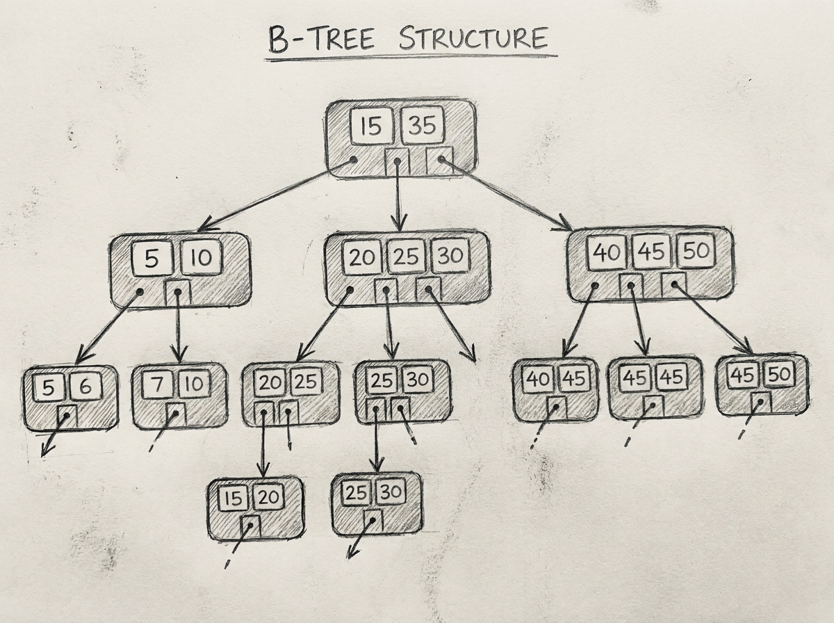
Structure of a B-Tree
Example:
          [20 | 40]

       /       |       \

 [5 | 10]  [25 | 30]  [50 | 60]
Properties:
- Keys inside nodes remain sorted
- Child subtrees maintain ordered ranges
- All leaf nodes remain at same depth
This guarantees balanced traversal.
How B-Trees Solve Problems of Binary Trees
Binary trees suffer from:
1. Large Tree Height
Since binary nodes contain only one key:
Height increases rapidly
B-Trees reduce height dramatically by storing many keys per node.
Example:
Instead of:
10 → 20 → 30 → 40
B-Trees may store:
[10 | 20 | 30 | 40]
inside one node.
This drastically reduces traversal depth.
2. Excessive Disk I/O
Storage systems transfer data in blocks/pages.
Reading one node at a time wastes disk bandwidth.
B-Trees align naturally with:
- disk pages
- memory pages
- storage blocks
Each node is intentionally designed to fit page sizes efficiently.
This minimizes disk operations.
3. Poor Scalability of Binary Trees
Large-scale databases may store:
- millions
- billions
- trillions
of records.
B-Trees maintain very small heights even for enormous datasets.
Example:
A B-Tree with large branching factors may store millions of entries with height only:
3 or 4
This makes searching extremely efficient.
How Searching Works in B-Trees
Suppose node:
[10 | 20 | 30]
Searching for 25:
- compare against keys
- determine correct interval
- descend into corresponding child
Traversal becomes:
Large jumps between ranges
instead of one-by-one node traversal.
Insertions in B-Trees
When inserting:
- keys are placed into correct node
- nodes split if capacity becomes full
- balancing occurs automatically
Example:
Before split:
[10 | 20 | 30 | 40]
After inserting 25:
[10 | 20 | 25 | 30 | 40]
If node exceeds capacity:
- median key moves upward
- node splits into two parts
This keeps the tree balanced.
Advantages of B-Trees
1. Extremely Low Tree Height
Because nodes store many keys:
- traversal depth remains very small
- searching becomes efficient
- disk access decreases dramatically
This is the biggest advantage of B-Trees.
2. Optimized for Storage Systems
B-Trees are specifically designed for:
- databases
- file systems
- indexing engines
- SSD/HDD storage
They align naturally with page-oriented storage architecture.
3. Efficient Insertions and Deletions
Operations remain logarithmic even for massive datasets.
Automatic balancing ensures consistent performance.
4. Excellent Scalability
B-Trees efficiently scale to enormous datasets without severe performance degradation.
This is why modern databases rely heavily on them.
5. Balanced Structure
All leaf nodes remain at same depth.
This prevents degenerate worst-case behavior seen in ordinary binary trees.
6. Reduced Disk Reads
Since one node contains many keys:
- fewer node traversals occur
- fewer page loads are needed
- I/O overhead reduces significantly
Limitations of B-Trees
Despite their strengths, B-Trees also introduce trade-offs.
1. Complex Implementation
Compared to:
- arrays
- linked lists
- binary trees
B-Trees require sophisticated logic for:
- node splitting
- merging
- redistribution
- balancing
Implementation becomes significantly more complicated.
2. Higher Memory Overhead
Each node stores:
- multiple keys
- multiple child pointers
This increases metadata overhead.
3. Less Cache-Friendly Than Arrays
Although efficient for storage systems, arrays still outperform B-Trees in pure in-memory sequential traversal because arrays maintain perfect contiguity.
4. Small Datasets May Not Benefit
For small data sizes:
- complexity overhead dominates
- simpler structures may perform better
Introduction to B+ Trees
As databases evolved further, another optimization became important:
Sequential range traversal.
Traditional B-Trees store records in both:
- internal nodes
- leaf nodes
This complicates efficient sequential scanning.
To solve this, B+ Trees were introduced.
What is a B+ Tree?
A B+ Tree is an advanced variation of a B-Tree where:
- internal nodes store only keys
- actual records exist only in leaf nodes
- leaf nodes are connected sequentially
Example conceptual structure:
Internal Nodes:
[20 | 40]

Leaf Nodes:
[5 10 15] ⇄ [20 25 30] ⇄ [40 50 60]
Leaf nodes form a linked sequence.
How B+ Trees Improve Upon B-Trees
B+ Trees introduce several major improvements.
1. Better Range Queries
Since leaf nodes are linked sequentially:
20 → 25 → 30 → 35 → 40
range traversal becomes extremely efficient.
This is highly important in:
- databases
- indexing engines
- ordered storage systems
2. Higher Branching Factor
Internal nodes store only keys, not full records.
This allows:
- more keys per node
- wider branching
- even smaller tree height
This improves scalability further.
3. Better Sequential Access
B+ Trees are optimized for sequential scanning.
This makes them ideal for:
- SQL range queries
- ordered iteration
- index traversal
4. Uniform Search Path
In B+ Trees:
- all actual records are stored at leaf level
- every search reaches leaf nodes
This creates predictable traversal behavior.
Advantages of B+ Trees
1. Excellent Range Query Performance
Leaf-level linked traversal enables highly efficient sequential access.
2. Better Disk Efficiency
Higher branching factors reduce tree height even further.
3. Widely Used in Databases
B+ Trees dominate modern storage systems including:
- MySQL
- PostgreSQL
- NTFS
- HFS+
- SQLite
because of their exceptional storage efficiency.
4. Efficient Ordered Traversal
Sequential leaf linkage makes iteration extremely fast.
Limitations of B+ Trees
1. More Complex Structure
Compared to ordinary B-Trees, B+ Trees require additional management of:
- linked leaves
- internal separation
- node balancing
2. Slightly Larger Traversal for Exact Search
Since actual records exist only in leaf nodes:
- exact searches always descend fully
whereas B-Trees may terminate earlier.
3. Higher Maintenance Complexity
Insertions/deletions involve:
- splits
- merges
- leaf linkage maintenance
This increases implementation difficulty.
When Should You Prefer B/B+ Trees?
B/B+ Trees are highly suitable when:
1. Massive Datasets Are Involved
Especially when data cannot fit entirely in RAM.
2. Disk I/O Optimization Matters
These structures are specifically engineered for minimizing storage access overhead.
3. Ordered Queries Are Frequent
Particularly:
- range searches
- sorted traversal
- indexed retrieval
4. Database or File-System Development
B/B+ Trees are foundational structures for:
- database indexes
- file systems
- storage engines
5. Scalability is Critical
They maintain efficient performance even at enormous scales.
When B/B+ Trees Are NOT Recommended
B/B+ Trees are not ideal when:
1. Dataset is Small
Simpler structures often outperform due to lower overhead.
2. Pure In-Memory Sequential Processing Dominates
Arrays may still provide superior cache efficiency.
3. Implementation Simplicity is Important
B/B+ Trees are substantially more difficult to implement correctly.
4. Frequent Random Pointer-Based Structures Are Sufficient
For simpler dynamic structures, linked lists or hash tables may be preferable.
B/B+ Trees: Foundations of Modern Storage Systems
B/B+ Trees combine several critical design goals:
| Capability | Source |
|---|---|
| Logarithmic search | Balanced trees |
| High branching factor | Multi-way nodes |
| Efficient storage access | Page-oriented design |
| Ordered traversal | Tree structure |
| Sequential range scanning | B+ leaf linkage |
They represent one of the most important breakthroughs in storage-oriented data-structure engineering.
Modern databases, file systems, indexing engines, and storage architectures rely heavily on B/B+ Trees because they align exceptionally well with real hardware behavior.
They demonstrate an essential systems-design principle:
Optimizing for disk and memory hierarchy is often more important than optimizing only CPU operations.
Conclusion
The evolution of data structures reflects one fundamental reality of computer science:
No single data structure is universally optimal.
Every structure is designed around specific trade-offs.
Static arrays introduced:
- simplicity
- contiguous memory storage
- extremely fast random access
but struggled with:
- fixed sizing
- costly insertions/deletions
- resizing limitations
Linked lists improved flexibility through dynamic allocation and efficient modifications, yet introduced:
- slow searching
- poor cache locality
- pointer overhead
As systems became larger and more performance-sensitive, hybrid structures emerged to bridge these gaps.
Dynamic arrays improved array flexibility through automatic resizing.
Skip lists introduced probabilistic shortcut traversal to achieve near-logarithmic performance while preserving linked-list simplicity.
Unrolled linked lists optimized memory locality by grouping multiple elements into block-oriented nodes.
B/B+ Trees revolutionized large-scale storage systems by minimizing disk I/O and reducing traversal depth through multi-way branching.
Each of these structures represents an attempt to balance competing goals such as:
- speed
- memory efficiency
- scalability
- hardware utilization
- insertion flexibility
- search performance
An important observation emerges from studying these structures:
| Problem | Preferred Design Philosophy |
|---|---|
| Fast indexing | Arrays |
| Dynamic modifications | Linked Lists |
| Balanced search + updates | Skip Lists |
| Better locality + flexibility | Unrolled Linked Lists |
| Large-scale storage systems | B/B+ Trees |
This demonstrates that data-structure design is fundamentally an exercise in engineering trade-offs.
Modern systems rarely rely on simplistic textbook structures alone.
Instead, real-world software often combines:
- cache-aware layouts
- probabilistic balancing
- hierarchical indexing
- block-oriented storage
- concurrent optimization
to achieve practical scalability and performance.
Another critical insight is that:
Hardware behavior strongly influences modern data-structure design.
Factors such as:
- CPU cache locality
- memory fragmentation
- disk access latency
- page-oriented storage
- parallel execution
have become just as important as asymptotic time complexity.
This is why many theoretically similar structures perform very differently in practical systems.
Ultimately, understanding these data structures is not merely about memorizing operations and complexities.
It is about understanding:
- why a structure exists
- what limitations it attempts to solve
- which trade-offs it introduces
- where it performs best
- where it becomes inefficient
The deeper one studies data structures, the clearer it becomes that:
Advanced data structures are essentially carefully engineered compromises between competing system constraints.
This is what makes data-structure design one of the most fascinating intersections of:
- algorithms
- hardware architecture
- operating systems
- memory management
- storage engineering
- real-world software scalability
Understanding these ideas provides the foundation for designing efficient systems, scalable software, high-performance databases, and modern computing infrastructure.